Comparing classifiers on the MNIST Data Set
This is a adaptation of a report written in collaboration with Louisa Lee (with some modfications) from my Machine Learning class in Fall 2017.
Introduction
The MNIST data set is a widely popular database of handwritten images of digits 0-9 for use in machine learning applications. More information about the MNIST set can be found here. All the images are stored in a specialized format. A helper file to parse the dataset was provided by the professor.
There are 60,000 total images in the dataset. The table below shows the number of images for each digit 0-9.
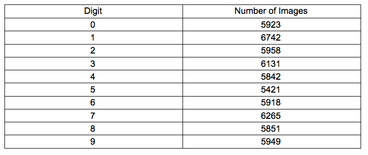
One benefit of the MNIST dataset is that strikes a decent balance in terms of the size of the problem. There are only 10 possible classifications and the images are relatively small at 28x28 pixels. However, just because the images are small does not mean that there is not large variance in the digits in the data set. Unsurprisingly, some of the digits are difficult to classify exactly straightforward for a human to correctly classify.
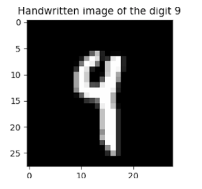
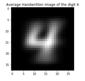
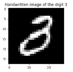
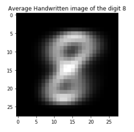
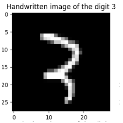
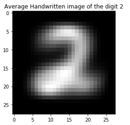
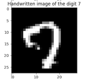
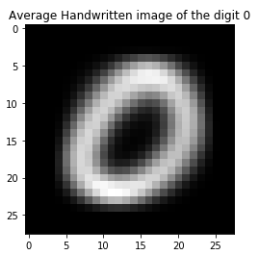
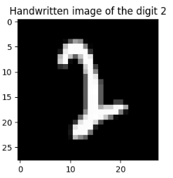
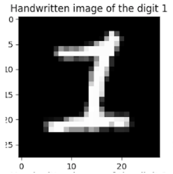
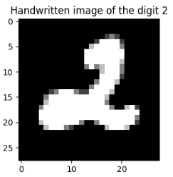
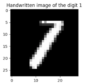
A selection of images that are likely to be very difficult to recognize with a classifier are shown next the composite average of the class the classifier is likely to pick. These images are difficult because they look extremely similar to the average (or another relatively common) image of another number. With a given distance metric in 10-dimensional space, a number that appears very similar to another number will have a relatively low distance to the cluster belonging to another class. Numbers such as these may be easily placed on the incorrect side of the decision boundary depending on the hyperparameters of the model in question.
| Image Likely to be Misclassified | Likely Misclassification |
|---|---|
 |
 |
 |
 |
 |
 |
 |
 |
 |
 |
 |
|
 |
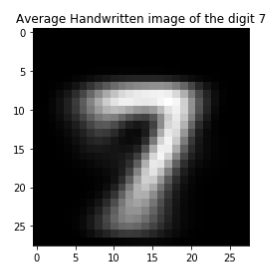 |
Table 1: Easily Misclassified images from the MNIST dataset
Both the training and testing sets were chosen as a set number of images for each digit label. For example, 3000 images per digit were used for the training set and 1000 images per digit as the validation set. This would result in 30,000 images in our training set and 10,000 images in our testing set. This method allows for good generalizability because it is predetermined that every digit is encompassed in the training and testing data. The training and testing data has an equal amount of images for each digit, allowing the training data to encompass all the possible labels and the testing data to reflect the classifiers performance on all numbers. Given that the training data set consists of 30,000 images and the testing set consists of 10,000 images, it was decided that N-fold cross-validation of the models was both too expensive in terms of time and not strictly required due to the amount of data available for both training and testing.
Even the relatively small 28x28 images provide lots of room for variance in the location and orientation of the digits drawn in the images. To help normalize the images, the MNIST images are centered. A major advantage of this normalization is that it will reduce the variance of the type of images a classifier may encounter. If all the images are centered and oriented correctly, the classifier does not need to learn how to account for those transofmations in its decision boundary. This also has the effect of reducing the
One major advantage of the taking this subset of the data in this manner is that it will reduce the variance in the images that the classifier sees. For example, if all the images are centered and rotated to appear perfectly vertically, the classifier does not need to learn to account for these transformations itself. If all the images are centered, it reduces the possibility that the classifier has “cheated” and just learned to look in a single area for a defining feature. However, this has the trade-off that the classifier has not really learned to identify the digit in general, it has only learned to classify digits that are close to the perfectly arranged data of the training set.
Suport Vector Machines
A support vector machine (SVM) is a type of supervised learning algorithm. The SVM will try to define an equation for a hyperplane in n-dimensions (where n is the number of dimensions in the data) to separate all the given examples of a class. To determine where this hyperplane should go, SVMs will try to maximize the margin between the data and the hyperplane. To solve non-linear problems, a kernel function can be applied to transform the data into higher dimensional space. Since the end-user need not know about this details of this step, only the points that effectively determine the decision boundary are returned. These points are called the support vectors.
To use an SVM for image classification, the image must be converted into a vector and passed to the SVM function. Given a certain dataset, the training process establishes the support vectors that define the decision boundary. By comparing the distance between an unknown input and these support vectors, the class of the new data point can be determined.
The slack hyperparameter for an SVM changes it from a hard-margin classifier to a soft-margin classifier. With a hard-margin, the hyperplane will adjust exactly to correctly identify all data points in the training set. For datasets that aren’t separable in n-dimsions, this will not terminate. A soft-margin classifier allows for misclassifications within a certain tolerance, otherwise known as slack.
The slack value determines if the occasional outlier is allowed to be on the wrong side of the decision boundary. This technically hurts the performance on the training data, but the hope is that it will lead to a more generalizable model by reducing the overfitting to the training data. This slack parameter is defined as C in sci-kit-learn. As C increases the model is forced to classify more and more of the training examples correctly.
SVMs can also use different kernel functions, some of which have additional hyperparameters. For this project, the radial basis function was used as the SVM’s kernel. This function takes an additional hyperparameter gamma. The impact of the gamma parameter defines a “radius of influence” for each support vector. A small gamma value extends this radius to much of the training set and approximates a linear classifier (see more here). Thus, finding the correct balance of C and gamma is an important task in generating a support vector machine model.
K-Nearest Neighbors
KNN is a method of supervised learning. The way KNN classification works is that it encodes the data into a vector and plots it in some n-dimensional space. Given an unknown data point, a given distance metric can be used to determine what the nearest k classified points are. From this set of k neighbors, the identity of the unknown point will be assigned as the majority opinion of those k neighbors. For the purposes of image classification, the same procedure applies. First, the image is converted into a vector and then compared against the k vectors nearest it. The most common resultant class is the predicted class of the new image.
The hyperparameter K in KNN determines how many neighbors to consider in the classification. When the K value is too small, it will fit the unknown data point to noise in the dataset (overfit), and when the K value is too large, it can make decision boundaries in the classification indistinct (underfit).
Derivation of the experiment
To determine an effective trade-off between training set size and exection time, the model accuracy as a function of the training size was determined.
Determination of the size of the training set
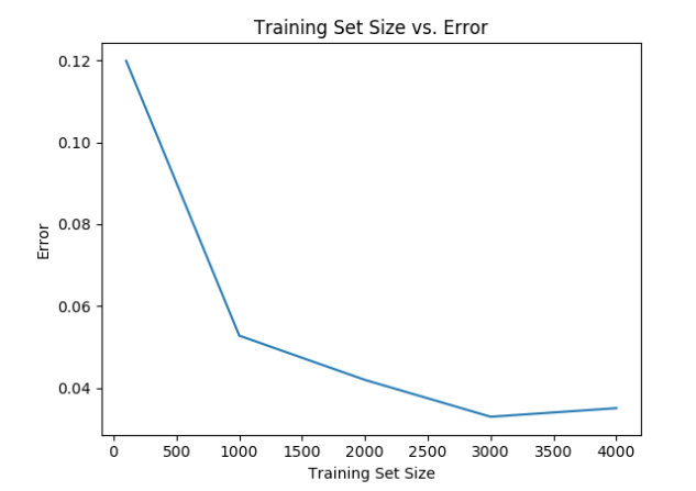
While holding the values of the hyperparameters C and gamma to a constant value, and with a constant testing set size, the size of the training set was varied. For this experiment C was left at default (1.0) and gamma was set to 0.035. The size of the testing set was kept at 1000 images per class, for a total of 10,000 images. The plot below shows the impact of the size of the training data set (per image class) on the error rate (y-axis.)
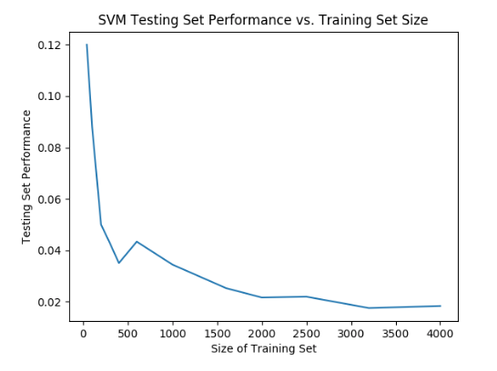
As the size of the training set increases toward 2000 images per class, there are substantial improvements in the model accuracy. After the 2000-3000 images per class range, the returns diminish rapidly. Thus, it does not make sense to train the SVM on more than a total of 30,000 images especially with the amount of time required to train the model.
The exact values of the hyperparameters for slack and gamma have a signficant impact on the peformance of the model. Initially, an exponential range of values were tried for each parameter independently until an approximate order of magnitude that performed decently was established. It so happened that the best approximate size was the values used to generate the plot in the previous part.
For both hyperparameters C and gamma a list was generated that included approximately +/- 20% of the values tried in the previous part. Since the parameters C and gamma are independent of each other, all \(O(N^2)\) of these combinations will be evaluated. This was achieved with 2 nested loops to iterate through the established trial values of C and gamma. On each loop iteration an SVM was trained and its accuracy on the testing set was computed. The result of this experiment is plotted in the graph below:
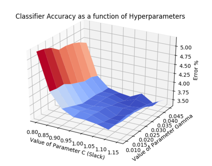
From this experiment, the best values of C was 1.15 and gamma=0.04 with an error rate of 3.52%. To accomplish this hyperparameter grid-search in a reasonable amount of time, the size of the training data was reduced to 1000 images per class (10,000) total. This explains the increase in error as compared to the 3000 images per class point in the previous experiment. Trading off 1.5% accuracy in training resulting in significantly less time to perform the entire experiment.
SVM Resuts
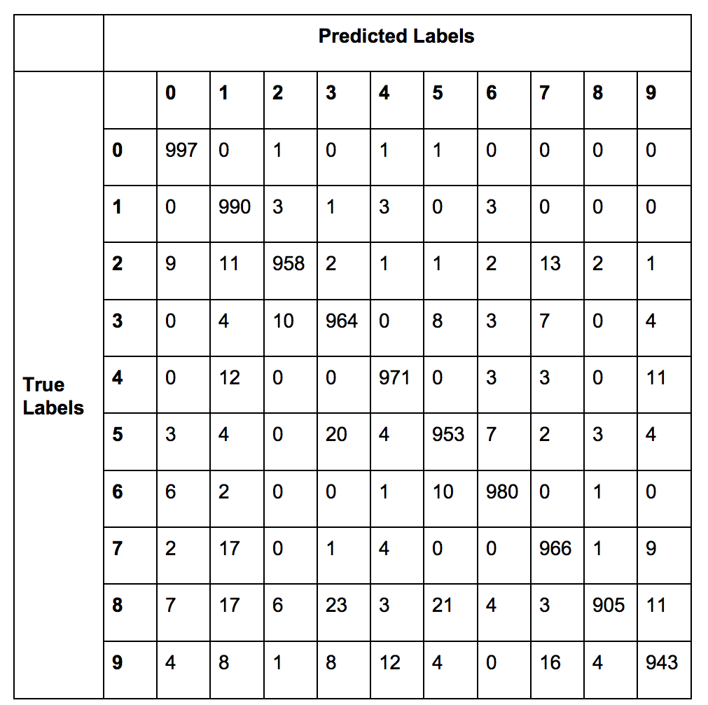
The table shown below is a confusion matrix of the SVM classifier with the hyperparameter values of \(C=1.15\) and \(\gamma=0.04\). The overall accuracy of the classifier was 97.18%. The confusion matrix is a useful evaluation tool as it also shows the predicted labels for all images in testing set.
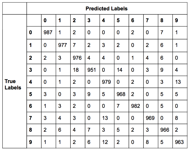
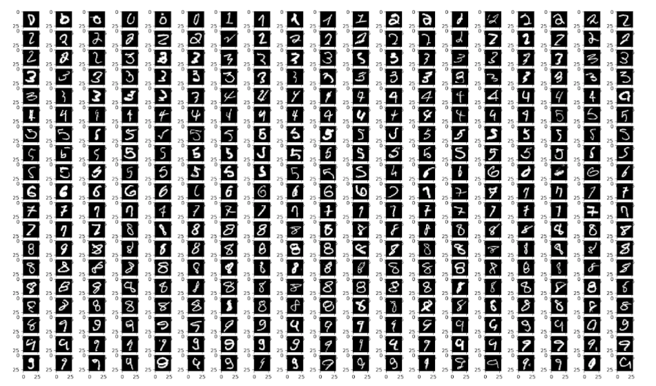
While 2.82% error is fairly good, it would be helpful to know if the testing images that were predicted incorrectly are actually hard for people to determine as well. The image below shows all images from the testing set for which the SVM classifier predicted incorrectly.
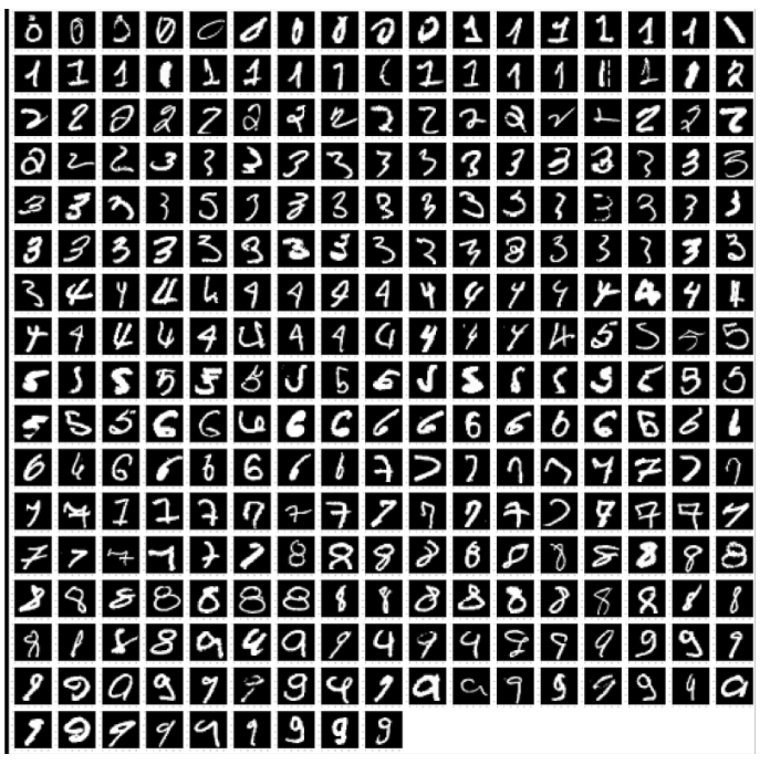
As anticipated, a significant proportion of the images that appear in the above plot are relatively similar in appearance to other numbers. There are multiple images that would even be reasonable for a human to misclassify if it were given randomly (for example: some of the 9s in the second to last row.) However, these lists as well as the confusion matrix reveal that there is not a significant trend in the misclassification. With the exception of 4 and 9, it seems that there is not a regular pattern in the predicted class when an image is misclassified.
Determination of KNN Hyperparameter
For the KNN classifier, the same setup of evaluating training set size was used. Initially, 5 neighbors (K=5) and a testing size of 1000 images from each number were used, resulting in a total of 10,000 testing images. The size of the training set was from 100-4000 images for each number 0-9 and the error rate was measured. The result is shown in the graph below.
As with the SVM, 3000 images per class seemed to result in the lowest error rate.
To determine the optimal number of neighbors to consider, the value of K was varried from 1 to 30 neighbors. The results are shown in the graph below:
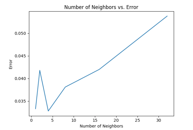
From the graph, it can be seen that 4 neighbors seems to be the optimal number of neighbors for the KNN classifier. This was found keeping the training size at 3000 images per number and the testing size at 1000 images per number.
Other parameters that were kept constant are the weights and distance measure. The weights were kept uniform so that all points in each neighborhood were weighted equally. The distance measure used was minkowski with p = 2, which is the equivalent to the standard Euclidean metric.
KNN Results
The resulting confusion matrix is shown below. The overall error rate of the model was 3.73%.
The images that were misclassified are shown below:
The images that were misclassified are largely ones where the handwritten digit is very similar to the average images of another number. For example, the 0 written in row 1 column 2 looks very similar to a 6. This shows that the KNN classifier is finding the images already classified from the training data that is most similar to the testing image. By using the nearest neighbor method, you find an already labeled image that is “closest” in terms of some distance measure and use that to label the unknown image. This relates to the section “Exploring the dataset” because the misclassified images are handwritten images that look very similar to another digit. As a result, this image will be nearer to the wrong labeled image than an image with its true label, resulting in the misclassification.
Discussion
Using a KNN resulted in an error of 3.73% with K=4 neighbors and a training size of 30,000 and testing size of 10,000. The support vector machine constructed resulted in an error of 3.52% with C=1.150000 and gamma= 0.040000 using the radial basis function as the kernel. To find an optimal hyperparameter for the KNN is an \(O(N)\) process, whereas finding the combination of both hyperparameters for the SVM is an \(O(N^2)\) process. For this reason even with a training size of 10,000 and a testing size of 1,000 the training process for the SVM takes considerably longer.
While the SVM performed slightly better than the KNN, it comes at the cost of significantly increased training time and the additional complexity of selecting a kernel function. However, once trained this disadvantage is not as much of an issue. By the fact that there were 2 independent parameters to be evaluated for the SVM, there is more granularity in adapting the SVM to solving this problem. Another likely reason for the SVM’s outperformance of the KNN has to do with how the hyperparameters function within the algorithm.
Consider a subset of numbers that are drawn very differently from the “normal” and appear very similarly to another digit: say 1s with a horizontal base for example. The nearest 5 neighbors to these outliers are likely to be the elements of another class (say 2), thus these would be misclassifications. However, depending on the tuning of the slack parameter, an SVM may be more likely to recognize this enclave of digits as belonging to belonging to class 1 instead of identifying them as members of class 2.
Boosted Classifiers
Boosting in a concept in machine learning that combines many cheap, weak, classifiers and uses them in coordination to solve tasks that would typically requrie an expensive strong classifier.
One algorithm for boosting is to use many decision stumps, (single question decision trees) to effectively provide constraints to define a hyperplane. This is the default option for the AdaBoostClassifier provided in scikit-learn.
AdaBoost Results
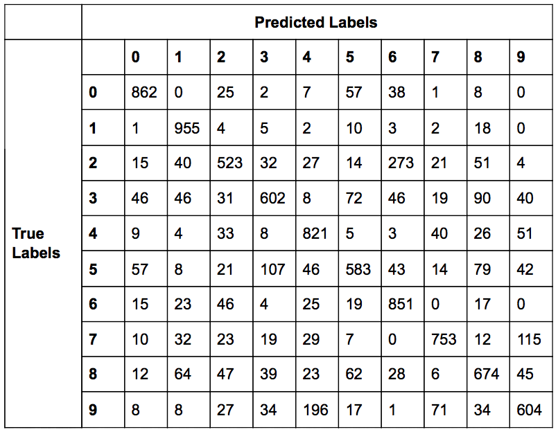
The results provided by the straightforward boosting implementation were not that impressive. The overall error rate was 27.72%. As shown in the confusion matrix below, there were several classes that were commonly misclassified as another class.
The AdaBoost algorithm is a meta-algorithm, that is it is an algorithm to apply on top of another algorithm. The results of boosting a SVM will be shown in the next section.
Boosting a SVM
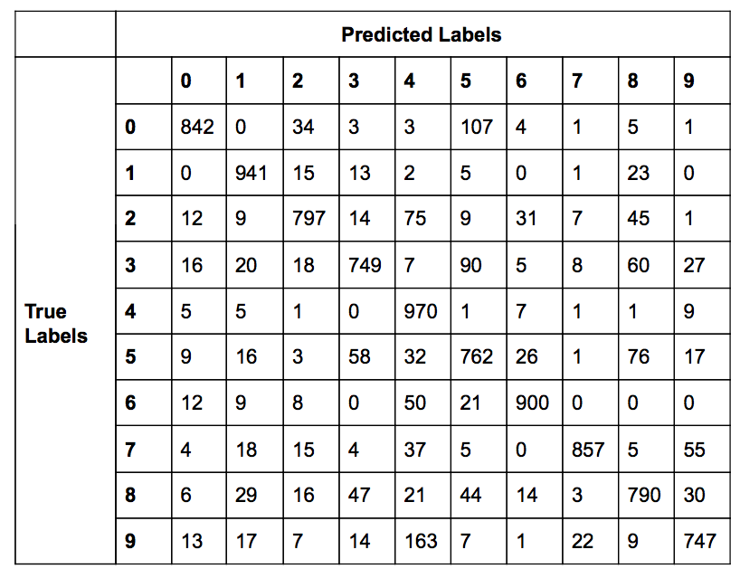
The SVM used with Adaboost used the radial basis function with \(C=1.15\) and \(\gamma=0.04\) as found previously. This boosted SVM had an error rate of 16.45%. This boosted classifier does not outperform either the SVM or the KNN as described previously (3.52%) and (3.72%) respectively. It should also be noted that an SVM with the linear kernel and the default C value was also tried. This variation of the classifier took less time to run the experiment and resulted in a very similar error rate of 16.21%. The data shown in the confusion matrix below is from the SVM trained with the radial basis function and \(C=1.15\), \(\gamma=0.04\).
Comparison of Boosted Classifier Results
The boosted classifier built with decision stumps had an error rate of 27.72% on the testing set. The boosted classifier built with a SVM had an error rate of 16.45%. By this metric alone, the Boosted SVM is far better than the boosted decision tree classifier.
Conclusion
The MNIST dataset provides an interesting problem that is both realistic and well constrained. 4 Different classifiers were analyzed in this report: a SVM, KNN, boosted decision trees, and a boosted SVM. The SVM had the lowest error rate of the classifiers tested, but this comes at the cost of an expensive process of hyperparameter tuning. The KNN performed almost as well with a very straightforward tuning process. The boosted classifiers did not perform well in this task. These days, Aritificial Neural Nets are frequently used in this kind of image recognition and classification tasks and many neural nets trained for the MNIST dataset often score in the 99th percentile range for classification accuracy. The SVM and KNN classifiers presented here a little behind this current state of the art, but still perform very well for their respective computational complexity.