The Fast-Fourier Transform and Spectrograms for Audio Visualization

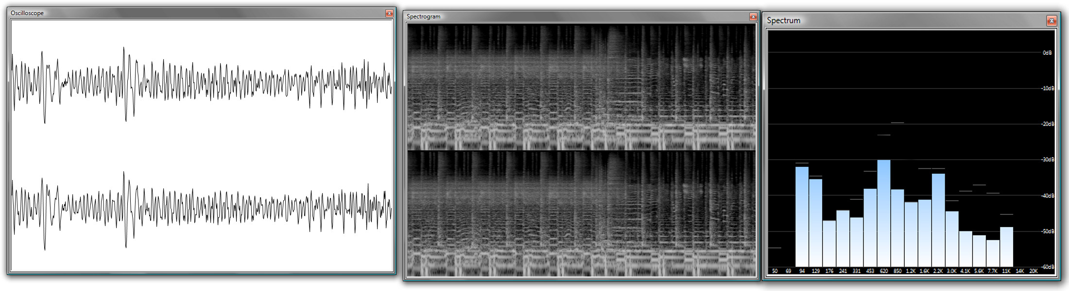
I started playing the Clarinet in 3rd grade, the Alto Saxophone in 7th, and soon after started working sound in my high-school’s AV Booth on everything from speeches to plays and large musical performances. At some point, I stumbled upon a music player called Foobar2000 and loved that it offered the same type of audio visualizations that were available to me in the booth. However, the spectrogram visualization was by far the most interesting. I loved trying to pick out individual instruments and their overtones and harmonics.

At the time, I had virtually no idea what it all meant, but after some discussion of Fourier Transforms in my first year of college, the math behind those visualizations started making some more sense.

The Main Idea

To put it in (relatively) simple terms, the Fourier Transform takes some input signal and outputs the respective weights of all the frequencies that compose the signal. For some signal, you could either

1. Record the entire signal, and then generate a single spectrum. Or,
2. Divide the signal up into chunks, and generate a spectrum for each chunk.

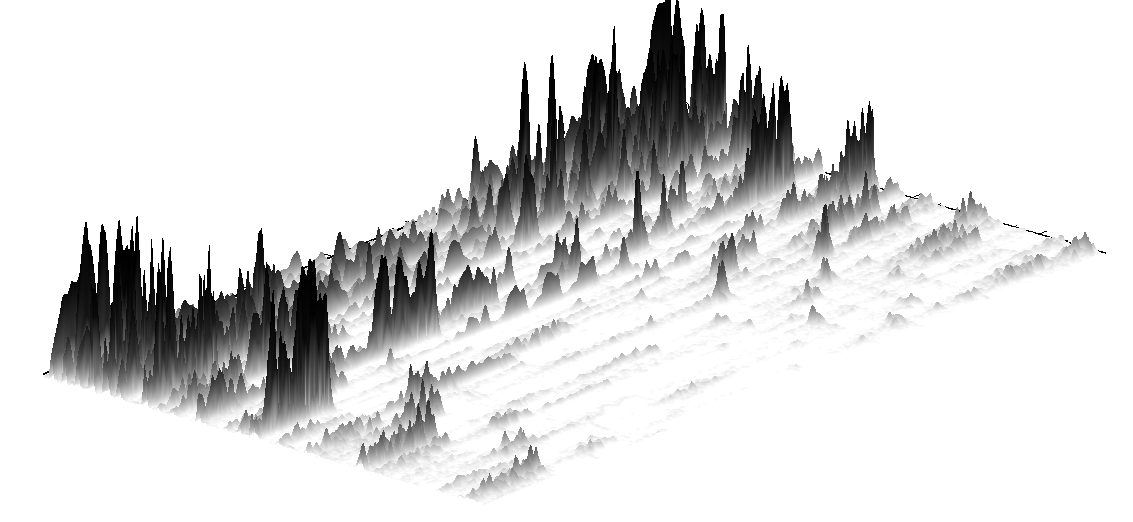
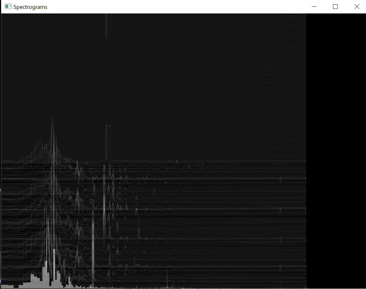
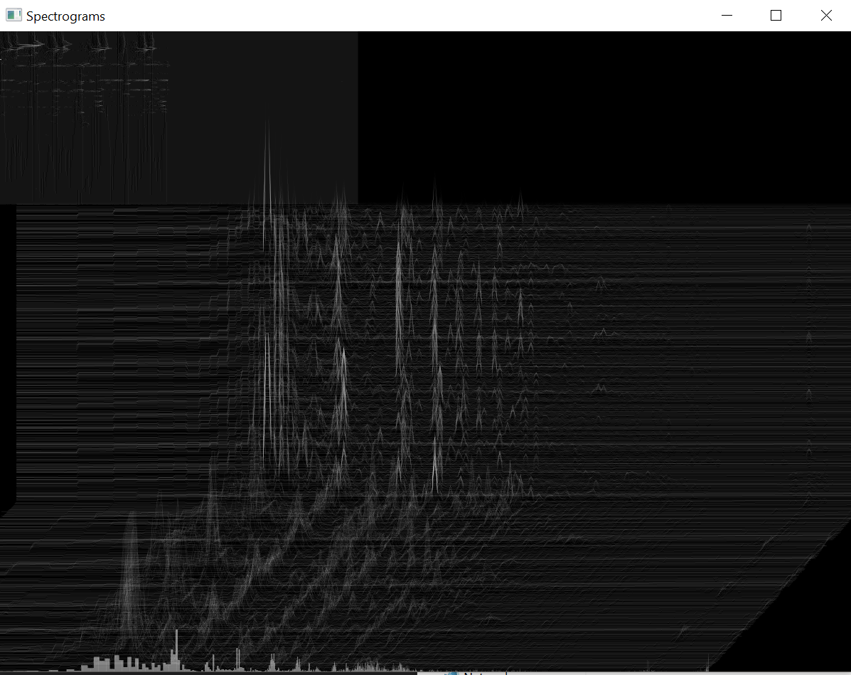
The first option may be useful for analysis, but for something even remotely close to real time, option 2 is the way to go. Since a spectrogram just a plot of frequency spectrum against time, we can essentially just line up each “chunk’s” spectrum to generate a spectrogram. It is pretty common in spectrograms to use color intensity to signify the amplitude of that frequency or frequency range, but I wanted to retain the typical spectrum plot and include the time dimension by offsetting the outline of the spectrum to give it a 3-dimensional look.

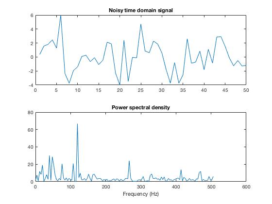
It’s practically trivial to generate a spectrum for an arbitrary signal in MATLAB (their tutorial here).

However, I decided against using MATLAB because I didn’t really want to spend lots of time trying to get it to plot the way I wanted it to. Instead, I decided to use C++ and a library to help me with the graphics. While it would be pretty easy to find a C++ library to also do the Fast-Fourier Transform for me like MATLAB can, I wanted to do some research into the algorithm and implement it myself since I am taking a signals and systems class in the Fall.

Fast-Fourier Transform

The naive approach to computing a discrete Fourier Transform results in an algorithm with \(O(N^2)\) time complexity. The complexity can be improved to \(O(N log(N))\) by using the recursive, divide and conquer, in-place Cooley-Tukey FFT algorithm. Next, I found a very helpful post on Stack Overflow with the pseudocode (the Wikipedia page’s pseudocode lines up more closely with the final version of my implementation.) With the pseudocode and some useful features of C++, implementing the algorithm is pretty simple.

1
2
3
4
5
6
7
8
9
10
11
12
13
14
15
16
17
18
19
20
21
22
typedef std::complex<double> ComplexVal; //short-hand for complex<double> representing a+bi
typedef std::valarray<ComplexVal> SampleArray; //array of complex-valued samples

void CooleyTukeyFFT::FFT(SampleArray& values) {
	const size_t N = values.size();
	if (N <= 1) return; //base-case

	//separate the array of values into even and odd indices
	SampleArray evens = values[std::slice(0, N / 2, 2)]; //slice starting at 0, N/2 elements, increment by 2
	SampleArray odds = values[std::slice(1, N / 2, 2)]; //slice starting at 1

	//now call recursively
	FFT(evens);
	FFT(odds);

	//recombine
	for(size_t i=0; i<N/2; i++) {
		ComplexVal index = std::polar(1.0, -2 * PI*i / N) * odds[i];
		values[i] = evens[i] + index;
		values[i + N / 2] = evens[i] - index;
	}
}

Initially, I had written my own helper function to handle dividing the array into even and odd arrays, but I found other implementations that used type definitions to clean up the type of the array and to allow usage of slice to greatly simplify splitting the arrays. I have adopted these modifications in my version. PI is just a #define constant in my .h file.

The Graphics Library

The next big task was figuring out how I wanted to do graphics for this project. One of the obvious choices for graphics with C++ was to use OpenGL, but I wanted to look the internet a bit before I committed to using a library. Luckily, I found SFML (Simple and Fast Multimedia Library). SFML not only handles the graphics side of things, but also nicely encapsulates important features like playing sound in a separate thread. Then, I found a YouTube video demonstrating a very similar Music Visualization tool to what I wanted to build that was also written using SFML. This project was quite close to what I wanted, so I started working on building a similar visualizer in SFML.

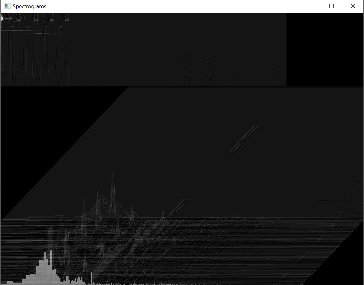
In lieu of having the oscilloscope view present in the video, I create an additional spectrogram more in the style of Foobar2000’s that can be toggled on and off with the space bar. For a library aimed at making games, I found it more than a bit strange that SFML did not have any built-in debouncing for key presses, so I had to write my own debouncing logic for the toggle. Toggling the modes also changes whether the time axis is at an angle or directly along the y-axis of the window.

I do also have some code to perform the inverse FFT. It certainly will not recreate the input signal exactly, but it would be fun to write out an audio file and hear just how distorted it is.